OK - we’ve drastically reduced the amount of work we have to do, so now let’s try to optimize what’s left as much as possible.

Series Overview

• Part 1 - What is the Mandelbrot set?
• Part 2 - What is the Buddhabrot?
• Part 3 - Algorithmic Optimizations
• Part 4 - Code Optimizations
• Part 5 - The Big Reveal

A note on benchmarks…

Benchmarks are hard.

There are three kinds of lies: lies, damned lies, and statistics benchmarks.

Jon Skeet, probably

Benchmarks in .NET are even harder - you’ve got the just-in-time compiler, the garbage collector, etc. Now, Jon Skeet might not have said the above, but he did work on the excellent BenchmarkDotNet project that makes some of the mechanics easier.

Even with tools like this, it can be pretty challenging coming up with realistic scenarios. When I dusted off my fractal code to prepare for my talk, some of the improved benchmarks I wrote didn’t remotely match what I had done just a year earlier (I think my earlier attempts were far too artificial). I can only say that the results I’m presenting are what I saw on my machine with my code. Your results may vary.

Break up processing

OK, back to tackling the big picture. The first concept is to break up the work into multiple stages:

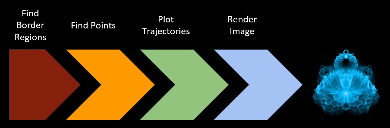
Unless you’re only making a teeny-tiny image, rendering a Buddhabrot is not something you want to do in a single step. The stages I used are:

• Find border regions - This doesn’t take too long, but it’s something we only have to do once.
• Find points - This is only finding points that match our iteration limit criteria. The output will be a bunch of complex numbers.
• Plot trajectories - Run through the points we found in the last step to find how many times each pixel location was visited. This stage will give us something of the same dimensions as the final image, but it’s just numbers at this point.
• Render image - Turn the raw numbers from the last stage into pretty pixels.

By breaking it up like this we can save our progress and easily add on to it. If we make a complete image and decide that we really need some more points, well, just find some more - the trajectory map from stage 3 can be added on to without recreating it from scratch. The last stage is likely the one that will be run the most number of times, since creating an aesthetically pleasing image is pretty subjective and there’s a lot of trial and error.

Stage 1 - Finding the border regions

It’s no surprise that some shortcuts get taken when you try to do a project in a weekend. Our initial attempt at find the border regions was a bit… suboptimal. Below you can see our old edge regions to the left, along with the newer version I made:

If you’re thinking to yourself “gee, the left side seems to include a lot more than just the edges” you would be absolutely correct. Since we didn’t bother visualizing what we had done, we didn’t notice there was a bug in the algorithm that caused it to spit out regions inside the set as well. It’s also far, far coarser than the new version I made (the right image is heavily shrunk down).

Having good border regions is key to making step 2 faster so it’s worth some time making sure the the borders you find are good. This is actually an area where it makes perfect sense to exploit the symmetry of the Mandelbrot set - the regions are going to be identical on both halves, so computing both sides is a waste. Of course, I only realized that part after I was done with it…

Stage 2 - Finding the points

Finding points that meet our criteria is by far the slowest part of the process, but it’s also the step with the most potential for optimization. The point search is what’s know as an embarrassingly parallel problem. There is no shared state that we have to keep track of, so every point calculation is entirely independent. The output of this stage is also very small - just a collection of starting points.

Thread-level parallelism

In .NET the easiest way for us to exploit parallelism is the Task Parallel Library, specifically the Parallel.Foreach construct. .NET will take care of distributing the work to different worker threads and managing that for you.

Honestly, I don’t have much to say about this - Ballmer-Jobs’ quote below sums it up. TPL is perfectly suited for this task.

Vectorization

Another form of parallelization that you might not be as familiar with is vectorization. To understand this we’re going to have to dive-down to the CPU instruction level:

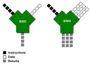
Most CPU instructions are what’s known as single instruction, single data (SISD). An instructions (like an ‘add’) works on one piece of data (ok, it might be two different variables) and produces a single output. With single instruction, multiple data (SIMD) instructions, the data and the output aren’t just a single scalar value but a vector of values. The ‘add’ instruction can now do multiple additions at the same time.

SIMD support was added to .NET 4.6 with the new RyuJIT compiler. To use it, you have to target x64-only and include the System.Numerics.Vectors NuGet package which exposes some SIMD-capable types. The CPU I ran the following benchmark on supports the AVX-2 instruction set which means it had 256-bit (32 byte) vectors to work with. Since a float is four bytes, we can cram 8 of them into a single vector for a theoretical speedup of 8x.

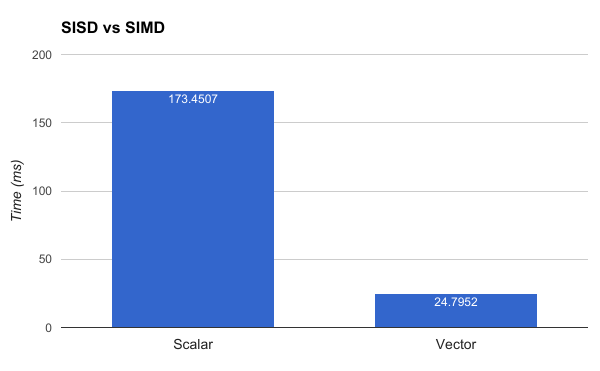
I’m not sure this benchmark is entirely accurate (I would guess the real-life speedup is somewhat less dramatic) but exploiting SIMD is a fantastic way to speed up the point search.

A final word I have on the subject is that vectorization is weird. There’s single-threaded code, multi-threaded code, and vectorized code as its own thing. For example, when calculating 8 points at once, they will probably meet the return condition at different times, but the loop has to keep going until all of them are done.

What about using a GPU?

The following is the die layout of a recent Intel CPU (I believe it’s the Skylake architecture):

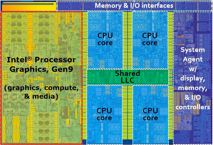
As you can see, this particular chip has 4 cores… along with a GPU that’s the same size as all of them combined! If you know anything about GPUs you know that Intel’s offerings are pretty modest as far as GPUs go, but even so they’re willing to devote that much expensive die space to it.

GPUs would be super-swell at finding points (churning through highly parallel data is their forté), but unfortunately the state of using GPUs in .NET isn’t great right now:

• CUDAfy.NET was a popular option (and it supported Intel GPUs) but it hasn’t had a release since April 2015. There seems to be about a dozen similar abandoned open-source projects.
• Alea GPU seems like a promising option. It’s commercially supported and was even featured on NVidia’s blog. Unfortunately, it’s NVidia-only and I don’t have one of those cards.

GPUs computing is something that I want explore but I just haven’t found the time for it yet.

Is Brent’s Algorithm worth it?

Remember this thing? Let’s actually measure the impact of using a cycle detection algorithm when finding Buddhabrot points:

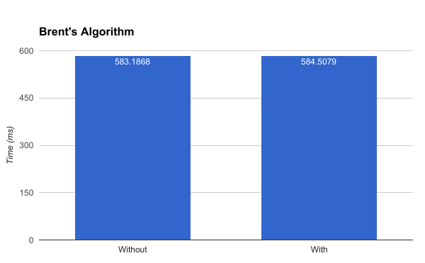
Welp.

To be fair, cycle detection is probably useful for other Mandelbrot scenarios, but in our case it’s kind of a dud.

Addendum 2017-05-16: I’m pretty sure I didn’t implement Brent’s Algorithm correctly. See my follow-up post for details.

Stage 3 - Plotting the points

Once we have a bunch of points, we need to plot their trajectories to generate the density map.

Our first approach used a bunch of int arrays to hold the map. This approach was ‘good enough’ for a 500 megapixel version - since an int is 4 bytes, that’s about 2GB of data. We actually did run into the dreaded OutOfMemoryException if we had too much other stuff running. Persisting it to disk was also relatively simple.

Clearly, that approach is not remotely scalable to 68.7 gigapixels.

• After (gasp!) examining the data, I decided that int was complete overkill and used ushort instead (unsigned 2-bytes).
• At 2 bytes per pixel location, that’s still a 128GB file. I used a memory-mapped file to hold this instead of messing around with arrays. This allows you to open an arbitrarily huge file and leave it up to the operating system to manage how much of it should be loaded into RAM (it’s essentially virtual memory).
• Instead of laying out the pixels in the same order as the final image (i.e. row by row), they were instead broken up into square subregions. This was for two reasons:
  • Each region was protected independently with a lock so that multiple threads could be used to compute trajectories. Since the order of the input points is essentially random, I hoped that they would (mostly) interact with completely different parts of the map to minimize contention overhead.
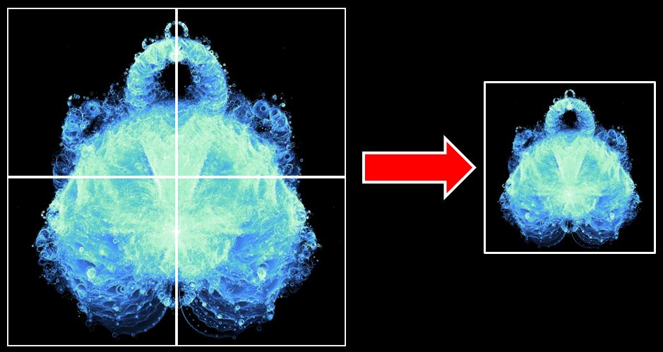
  • Each region is 256 x 256 pixels. This size corresponds with the tile size used in the next stage.

The above image shows the grid concept. The full size version used 1024 x 1024 regions.

Stage 4 - Generating the Image

Before we get into more details about how to display the output, we first need some way of turning the trajectory map (which is just a bunch of numbers) into colors.

Fit the data!

In our first attempts at generating the Buddhabrot we were essentially going blind - we had no idea what the data looked like so the algorithm was entirely trial-and-error. If you go down that route, your first attempts will probably resemble the left and right versions in the below image: either your image will be incredibly dim or utterly blown out. How do we get a Goldilocks image like in the middle?

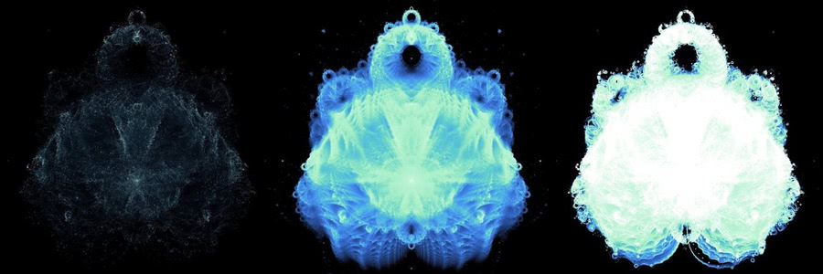
I eventually came upon the novel concept of examining the data inside the giant trajectory plot. By doing some simple histograms, it became clear that a vanishing small number of pixels were visited a tremendous number of times (around the origin, for example) while the vast majority of pixels had orders of magnitudes less hits. This distribution of data is what causes extremely dim images like the above left if you try to linearly map the hit counts to colors - the handful of locations with high hits will be the only bright parts. If you attempt to correct it too much to bring out the detail in the dim areas, the areas with greater counts will become blown out like in the right image. To get something better, we have to reduce the highs while bringing up the lows.

Tone Mapping

The eventual algorithm I came up with was informed by the histogram of the hit counts to try to balance the distribution of colors based on how many pixels fell into each range. After the fact, I realized that what I had done fell into the domain of tone mapping. Tone mapping is a process of converting high-dynamic data into a more limited range. Typically it is used for combining multiple photographs with different exposures to get the best of all worlds:

Using the parlance of tone mapping, what I had come up with was a global operator - every single pixel in the image was independently calculated. There is another class of tone mapping algorithms called local operators that also take into account the surrounding data.

I’m reasonably happy with my results but there are still some areas that don’t show a lot of detail. Playing around with some existing tone mapping algorithms (especially the local operator varieties) would be an interesting experiment.

RBG vs HSV

One recommendation I have is that anytime you’re doing actual computations with colors, do not use RGB.

Representing colors with red-blue-green components is simple to understand and fast for computers, but computing gradients with them can give pretty miserable results. Instead, something like hue-saturation-value is a much, much better alternative.

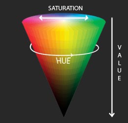
Linearly interpolating between two colors represented as HSV will give much more pleasing results than doing the same with RGB.

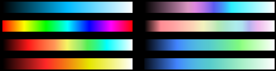
The Tyranny of Color Theory

Picking the colors you want is ultimately subjective, but you might run into issues with color perception. Human eyes are not equally sensitive to the entire color spectrum. Some colors will simply look brighter than others even though they are “mathematically” equal. This can be pretty frustrating if you’re trying to put together a palette that maximizes the use of color in order to show more detail. I experimented with a lot with different palettes before settling on the fairly conservative one in the bottom right corner:

Displaying the Output

Generating a single huge image file is only feasible up to a couple of hundred megapixels. We had already hit some kind of Windows limit with the first 500 megapixel version so a better solution was needed.

After exploring different deep-zoom options, the one that made the most sense to me was to use a web mapping library. Satellite views on things like Google Maps are the exact same concept as showing a large Buddhabrot rendering - a massive amount of image data that can be displayed at different zoom levels, where only the visible portion is loaded.

I used a framework called Leaflet to display the final result images. Each of the 256 x 256 regions from the trajectory map was converted to a tile image. Those tiles represent the deepest zoom level of the Buddhabrot. Map frameworks like Leaflet load different sets of images for the different zoom levels. 4 tiles would be represented by 1 when zoomed out a level.

To create the other zoom levels, I used ImageMagick to “glue” tiles together.

Originally I used PNG files as the output since it’s lossless, but the size was pretty unwieldy - around 45GB for all the tiles. I found that JPEGs at 80% quality setting looked almost indistinguishable but with a much more palatable final size of under 16GB (and that’s without Google’s new Guetzli encoder).

Image Mechanics - Beware of System.Drawing.Bitmap.SetPixel

The standard bitmap class in .NET only has one obvious way of setting colors: SetPixel. Unfortunately, SetPixel is brutally slow. The better way to do things is to use LockBits/UnlockBits and to directly manipulate the pixel buffer inside of the image. I’m not sure why they haven’t added a nicer convenience method to allow you to set all the colors at once, but it is very much worth your while to do things the hard way:

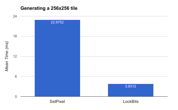
Remember that we’re generating 1,048,576 tiles (1024 x 1024) so the time savings from this change is nearly 5.6 hours!

Summary

So far we’ve learned:

• What the Mandelbrot set is
• What the Buddhabrot is
• How to reduce the amount of work involved through algorithmic optimizations
• How to speed up / implement the remaining work

Next time I’ll finally show off the big guy!